The relational model and skew lattices, Part I

So, how about noncommutative lattices in data science?

The aim of this post is to demonstrate a connection between data science and noncommutative lattices, more precisely skew lattices. This is work in progress.

The relational model is one of the most basic models used in data science. Data is organized into tables called relations, each being composed of rows and columns. Columns correspond to attributes, while rows correspond to data entries. Rows are often referred to as records. In data science, a database organized as a relational model can be manipulated for instance with the SQL (pronounce: "sequel") language. 

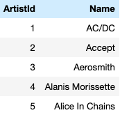
Let's look at an example. The open source Chinook database represents a digital media store with the media related data collected from the iTunes Library. It is composed of several tables like artists, albums, tracks, genres etc. In order to get some insight into the database, let's look at the first five records of the following tables: artists, albums, genres.

The artists table

The albums table

The genres table

With basic SQL operations we can extract information from the tables. For instance, knowing that Deep Purple has AritstId equal to 58, the following SQL command allows us to select all their albums:

SELECT * FROM albums WHERE ArtistId = 58;

The result is given in the table below:

All albums by Deep Purple.

Moreover, we can construct new tables from the existing ones by operations like union, intersection, difference, product or join (actually, several kinds of joins).

Examining the tables above, we see that artists is a very simple table with just two columns. The ArtistId column uniquely identifies each record of the table. Similarly, AlbumId uniquely identifies elements of the albums table. However, we see that the albums table also has a column corresponding to the ArtistId attribute -- with the values in this column denoting the author of the album. 

When we want to specify which table an attribute corresponds to, we write it in the form 

table.Attribute 

like albums.AlbumId. Assume that we want to create a table of albums together with the artists (with their names listed). What we can do is join the two tables. The (inner) join (with a pair of joining columns specified) of two tables returns a table with columns corresponding to all columns of the two tables (identifying the joining columns) and consisting of records having equal values in the joining columns. For instance, joining tables albums and artists on attributes albums.ArtistId = artists.ArtistId results in the table of all albums (AlbumId, Title, ArtistId) with the artists (Name); here the name of an artist is assigned to a record based on the ArtistId. 

First ten records of the join of tables albums and artists.

Not knowing the ArtistId of Deep Purple we could extract their albums using the following command:

SELECT * FROM albums JOIN artists ON albums.ArtistId = artists.ArtistId WHERE Name = "Deep Purple";

The resulting table is given below.

Table of albums by Deep Purple.

If we prefer to omit the two ArtistId columns from the result, we can change our command to:

SELECT AlbumId, Title, Name  FROM albums JOIN artists ON albums.ArtistId = artists.ArtistId       WHERE Name = "Deep Purple";

We obtain the following table:

Table of albums by Deep Purple.

Now we know a little bit about the relational model. How about skew lattices? Let's begin with an example. 

Consider sets A = {a, b} and B = {1, 2}, and let S be the set of all maps f: X → B, with the domain X being a subset of A. Then S contains the following maps:

Maps with domain X = ∅: just the empty map f₀ = ∅.

Maps with domain X = {a}: 

• f1 : a ↦ 0
• f2 : a ↦ 1

Maps with domain X = {b}: 

• f3 : b ↦ 0
• f4 : b ↦ 1

Maps with domain X = {a, b}: 

• f5 : a ↦ 0, b ↦ 0
• f6 : a ↦ 0, b ↦ 1
• f7 : a ↦ 1, b ↦ 0
• f8 : a ↦ 1, b ↦ 1

We see that S = {f0, ..., f8}.

The skew lattice S of partial functions.

Skew lattices have rich algebraic structure. For now, let's just consider the so called Green's equivalence relation D. Given a skew lattice of partial functions like the one above, partial functions f and g in S are said to be D-equivalent if and only if they are defined on the same domain, i.e. dom f = dom g. Let's visualize S once more, this time also depicting relation D:

Skew lattice S with D-classes.

Now, doesn't this look familiar? Indeed, we can interpret elements of S as records in a database, with D-classes playing the role of tables. Our "database" has four tables, each having a column for identification as well as columns corresponding to elements of the corresponding domain. Moreover, a record corresponding to a function f has value f(x) in the column corresponding to x. We obtain the following four tables:  

Table corresponding to the empty domain.

Table corresponding to domain {a}.

Table corresponding to domain {b}.

Table corresponding to domain {a, b}.

Of course, we could also drop the identification columns in the above tables. Then we would see that the table corresponding to the domain {a, b} is exactly the cartesian product of tables corresponding to domains {a} and {b}.

The above example illustrates that there appears to be a way to see the D-classes of a skew lattice as tables of a relational model. How about the converse? Let A = {a₁, ..., a_k} be the attributes of a table T. Then any record of T can be seen as a map from A to some set of values, assigning to a_i the value in the corresponding column. Hence we can view records of tables in a relational model as partial functions from the union of all the attributes of all the tables to some codomain. 

Moreover, there are joins both in the relational model and in skew lattices. How are these operations related? Let's talk about this in the next post.